Visualization

Overview

There are broadly two types of visualizations: box-based and halo-based, spanning all particle types and fields. There is no fundamental difference between the two, other than the fact that halo-based visualizations are centered on individual halos/galaxies, while box-based visualizations show a fixed region of the simulation volume, and the available options are somewhat specialized to these two cases. There are four main visualization functions:

• temet.vis.halo.renderSingleHalo() - halo/galaxy-centric visualization.

• temet.vis.halo.renderSingleHaloFrames() - generate a series of movie frames across snapshots in time.

• temet.vis.box.renderBox() - full box visualization.

• temet.vis.box.renderBoxFrames() - generate a series of movie frames across snapshots in time.

Users can call these functions directly. There are also a number of driver functions that show examples of setting up various common, to advanced, visualization configurations:

• vis.boxDrivers contains numerous driver functions which create different types of full box images.

• vis.boxMovieDrivers create frames for movies, including many of the available TNG movies.

• vis.haloDrivers as above, except targeted for images of individual galaxies and/or halos.

• vis.haloMovieDrivers generate frames for halo/galaxy-centric movies, including time/merger tree tracking.

The general approach, also followed in these driver functions, is to create a list of panels, where each entry in the list corresponds to one image/view/panel in the final figure. Each panel is specified by a dictionary of options, including the particle type, field to visualize, colormap, scaling, etc.

• Any option not specified in a panel will fall back to a common value, set as local variables in the driver function.

• Any option not specified in either the panel or the local variables will fall back to a default value.

Finally, global plotConfig settings affect the overall figure as a whole (e.g., layout, figure size, and so on).

Box-based visualization

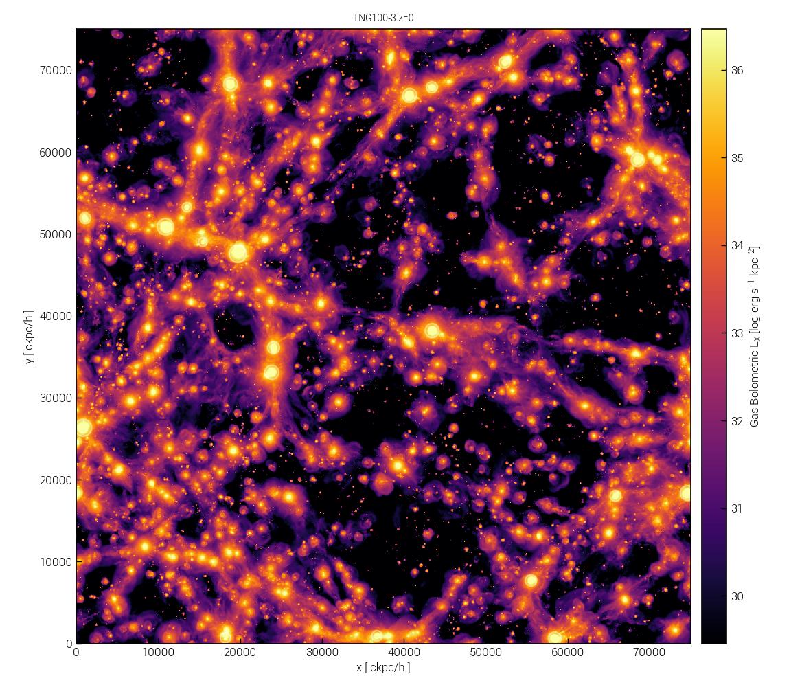
For example, we can render a single panel visualization of a cosmological box:

sim = temet.sim(run='tng100-3', redshift=0.0)

panels = [{'sP':sim, 'partType':'gas', 'partField':'coldens_msunkpc2'}]

temet.vis.box.renderBox(panels)

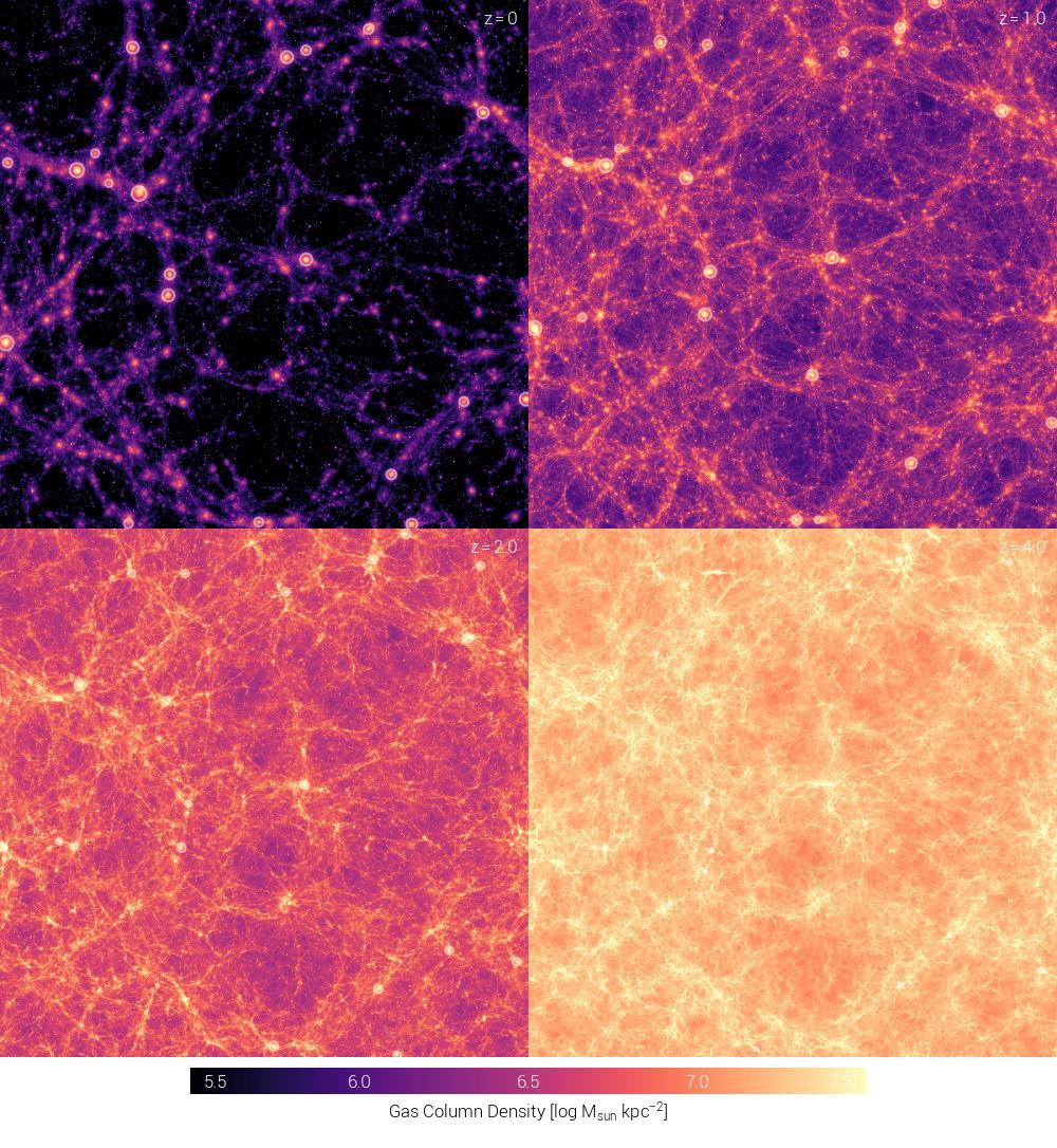
Multiple panels can vary any option. For instance, a 4-panel visualization at different redshifts:

sim = temet.sim(run='tng100-3', redshift=0.0)

config = {'plotStyle': 'edged'}  # overall figure config
common = {'labelZ': True, 'valMinMax': [5.5, 7.5]}  # common variables shared between all panels

panels = []

for z in [0.0, 1.0, 2.0, 4.0]:
    panels.append( {'sP':sim, 'redshift':z, 'partType':'gas', 'partField':'coldens_msunkpc2'} )

temet.vis.box.renderBox(panels, config, common)

The “edged” plot style is a custom, minimal layout that avoids the usual matplotlib axes and colorbars:

Tip

You can notice a number of white circles overlaid on the images above. These indicate the locations (and virial radii) of the N most massive halos. Specialized overlays and markers can indicate halos, satellite subhalos, SMBH locations, contours of other fields, and so on (see below).

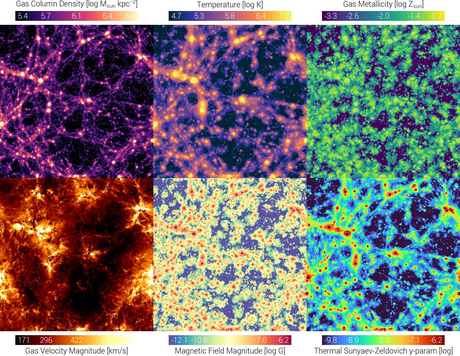
Or a 6-panel visualization comparing different fields:

sim = temet.sim(run='tng100-3', redshift=0.0)

config = {'plotStyle': 'edged'}  # overall figure config
common = {'sP': sim, 'partType': 'gas'}  # common variables shared between all panels

panels = []

panels.append({'partField':'coldens_msunkpc2'})
panels.append({'partField':'temp'})
panels.append({'partField':'metal_solar'})
panels.append({'partField':'velmag'})
panels.append({'partField':'bmag'})
panels.append({'partField':'sz_yparam'})

temet.vis.box.renderBox(panels, config, common)

Caution

In the above examples, we specified the simulation both in the common dictionary and in each panel. Either approach is valid; if specified in both places, the panel entry takes precedence. When panel values override common values, an informational warning is printed.

Note

The above examples use the default figure layout, which automatically arranges panels into rows and columns. Users can also specify a custom layout by setting plotConfig.nRows and plotConfig.nCols.

Note

The partField option can be any number of built-in or custom fields. See temet.vis.quantities for more information.

The partType option can be any valid particle type.

Tip

Many other options can be specified per-panel, including colormap, scaling, image size, and so on. See the API documentation for temet.vis.box.renderBox() for a full list of available options.

Halo-based visualization

For a halo-based render, the process is the same, and subhaloInd specifies the subhalo ID:

sim = temet.sim(run='tng50-1', redshift=0.0)
subID_a = sim.halo(50)['GroupFirstSub']
subID_b = sim.halo(51)['GroupFirstSub']

config = {'plotStyle': 'edged'}  # overall figure config
common = {'sP': sim, 'partType': 'gas', 'labelHalo':'mhalo,mstar,id'}  # common variables shared between all panels

panels = []
panels.append( {'subhaloInd':subID_a, 'partField':'coldens_msunkpc2'} )
panels.append( {'subhaloInd':subID_a, 'partField':'temp'} )
panels.append( {'subhaloInd':subID_b, 'partField':'coldens_msunkpc2'} )
panels.append( {'subhaloInd':subID_b, 'partField':'temp'} )

temet.vis.halo.renderSingleHalo(panels, config, common)

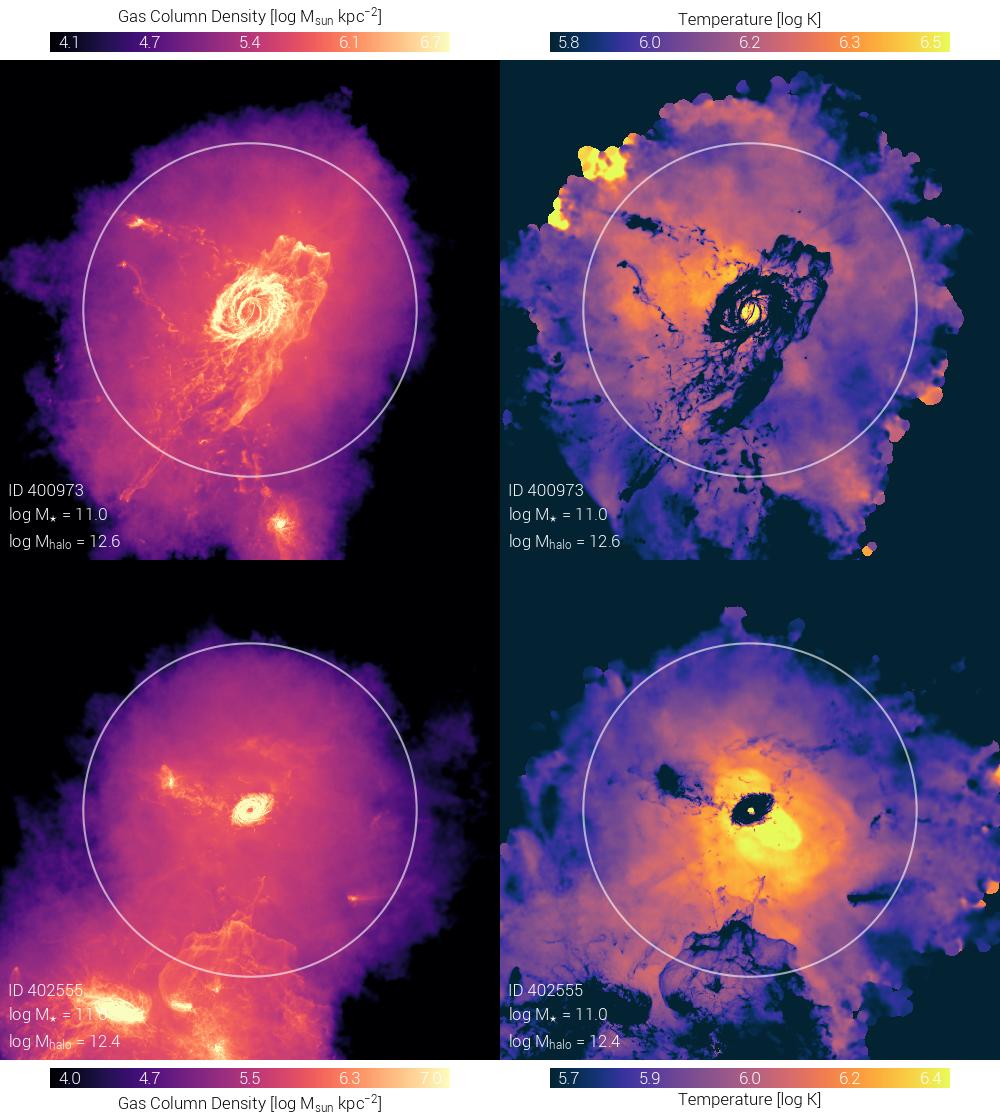
The white circle indicates the virial radius (\(R_{\rm 200c}\)) of the halo, by default. This can be customized.

Hint

You will notice that the renders become noisy and then have “blank” regions at larger radii, i.e. starting slightly beyond the virial radius. This is because the scope of the snapshot data used for the rendering is scope="fof" (by default), which only loads particles associated with FoF groups. This takes advantage of the snapshot structure of TNG-like data, where particles/cells are stored by halo, making it extremely efficient to load only this data. This can be customized, including scope="global" to use the entire snapshot.

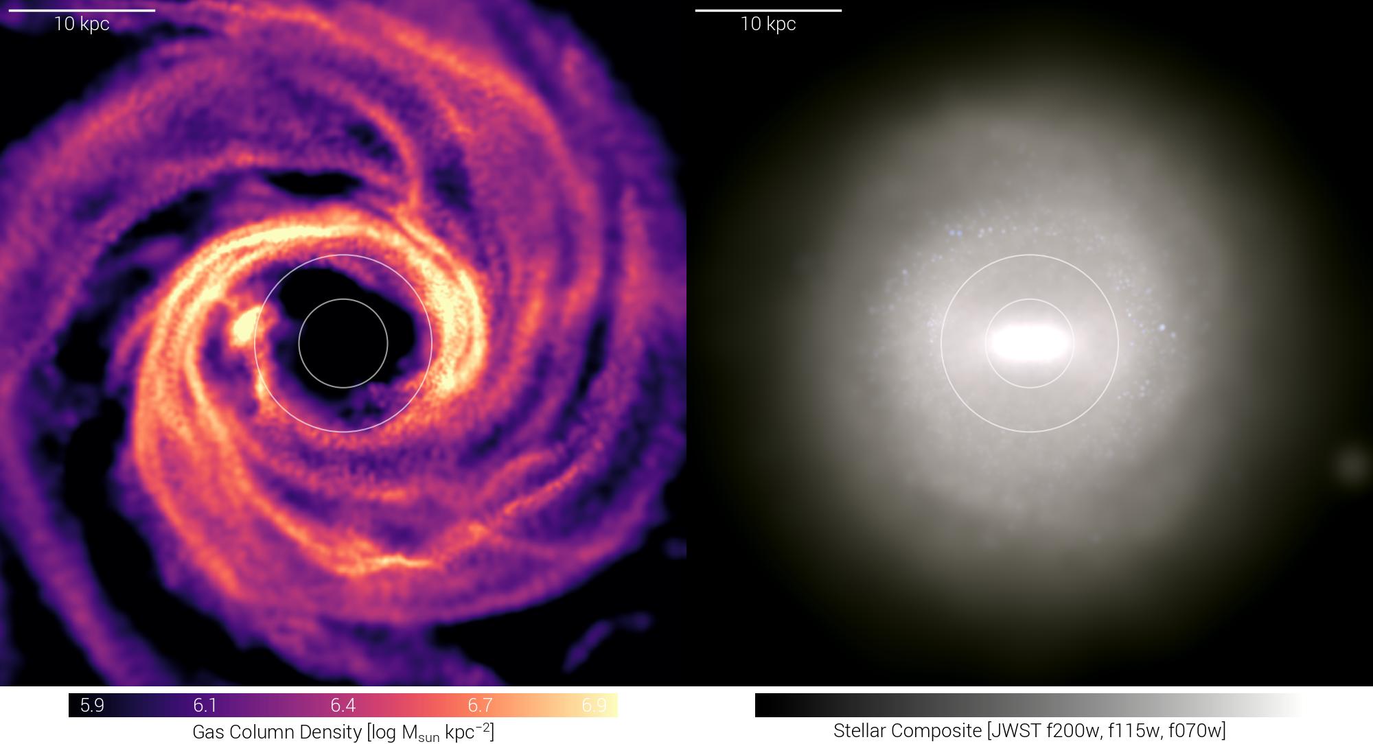
A common practice in the drivers is to use local variables for common configuration, e.g.:

# common (panel) options: all local variables are captured by locals() and passed to renderSingleHalo
sP = temet.sim(run='tng50-1', redshift=0.0)

subhaloInd = sP.halo(150)['GroupFirstSub']

labelScale = True
labelHalo  = True
size       = 50.0
sizeType   = 'kpc'
rVirFracs  = [1.0, 2.0]
fracsType  = 'rHalfMassStars'
rotation  = 'face-on'

# set overall figure config and make panels
config = {'plotStyle': 'edged'}

panels = []
panels.append( {'partType':'gas', 'partField':'coldens_msunkpc2'} )
panels.append( {'partType':'stars', 'partField':'stellarComp'} )

temet.vis.halo.renderSingleHalo(panels, config, locals())

Warning

Be careful using locals() to pass local variables to the rendering function, as this captures all local variables, which may include unwanted entries. Particularly in complex drivers, you may have variables whose names overlap with valid panel options, leading to unexpected behavior.

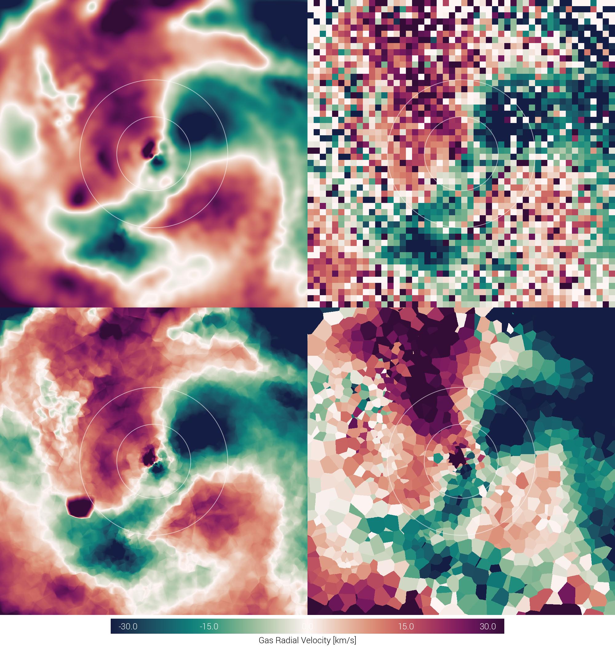
So far, we have always been using the default rendering method, that makes weighted-projections using an adaptive-size cubic (SPH-like) kernel. Other rendering methods are available, including simple 2D histograms, nearest-neighbor interpolation, Voronoi projections and slices, and others. For example:

# common (panel) options
sP = temet.sim(run='tng50-3', redshift=0.0)

subhaloInd = sP.halo(150)['GroupFirstSub']

size      = 50.0
sizeType  = 'kpc'
rVirFracs = [1.0, 2.0]
fracsType = 'rHalfMassStars'
partType  = 'gas'
partField = 'vrad'
valMinMax = [-30, 30]
rotation  = 'face-on'

# overall figure and panel setup
config = {'plotStyle': 'edged'}

panels = []
panels.append( {'method': 'sphMap'} ) # default
panels.append( {'method': 'histo', 'nPixels':[50,50]} )
panels.append( {'method': 'voronoi_proj'} )
panels.append( {'method': 'voronoi_slice'} )

temet.vis.halo.renderSingleHalo(panels, config, locals())

Configuration Options

A full list of available configuration options for both box-based and halo-based visualizations can be found in the documentation for temet.vis.box.renderBox() and temet.vis.halo.renderSingleHalo(), respectively. Broadly speaking, common options include:

sP:

(default: None) simulation instance (snapshot/redshift must be set)

hInd:

(default: None) halo index for zoom run

run:

(default: None) if sP is not input, simulation name (must also specify res and redshift)

res:

(default: None) if sP is not input, simulation resolution

redshift:

(default: None) if sP is not input, simulation redshift

partType:

(default: ‘gas’) which particle type to project

partField:

(default: ‘temp’) which quantity/field to project for that particle type

valMinMax:

(default: None) if not None (auto), then stretch colortable between 2-tuple [min,max] field values

method:

(default: ‘sphMap’) sphMap[_subhalo,_global], sphMap_{min/max}IP, histo, voronoi_slice/proj[_subhalo]

nPixels:

(default: [1920,1920]) [1400,1400] number of pixels for each dimension of images when projecting

ptRestrictions:

(default: None) dictionary of particle-level restrictions to apply

axes:

(default: [1,0]) e.g. [0,1] is x,y

axesUnits:

(default: ‘code’) code [ckpc/h], kpc, mpc, deg, arcmin, arcsec

vecOverlay:

(default: False) add vector field quiver/streamlines on top? then name of field [bfield,vel]

vecMethod:

(default: ‘E’) method to use for vector vis: A, B, C, D, E, F (see common.py)

vecMinMax:

(default: None) stretch vector field visualizaton between these bounds (None=automatic)

vecColorPT:

(default: None) partType to use for vector field vis coloring (if None, =partType)

vecColorPF:

(default: None) partField to use for vector field vis coloring (if None, =partField)

vecColorbar:

(default: False) add additional colorbar for the vector field coloring

vecColormap:

(default: ‘afmhot’) default colormap to use when showing quivers or streamlines

labelZ:

(default: False) label redshift inside (upper right corner) of panel {True, tage}

labelScale:

(default: False) label spatial scale with scalebar (upper left of panel) {True, physical, lightyears}

labelSim:

(default: False) label simulation name (lower right corner) of panel

labelHalo:

(default: False) label halo total mass and stellar mass

labelCustom:

(default: False) custom label string to include

ctName:

(default: None) if not None (automatic based on field), specify colormap name

projType:

(default: ‘ortho’) projection type, ‘ortho’, ‘equirectangular’, ‘mollweide’

projParams:

(default: {}) dictionary of parameters associated to this projection type

rotMatrix:

(default: None) rotation matrix, i.e. manually specify if rotation is None

rotCenter:

(default: None) rotation center, i.e. manually specify if rotation is None

Note

You can either specify sP (a simulation instance), or provide its name, resolution, and redshift (i.e. all the arguments to simParams).

Halo-render specific options include:

subhaloInd:

(default: 0) subhalo (subfind) index to visualize

rVirFracs:

(default: [1.0]) draw circles at these fractions of a virial radius

fracsType:

(default: ‘rVirial’) if not rVirial, draw circles at fractions of another quant, same as sizeType

rotation:

(default: None) ‘face-on’, ‘edge-on’, ‘edge-on-stars’, or None

mpb:

(default: None) use None for non-movie/single frame

cenShift:

(default: [0,0,0]) [x,y,z] coordinates to shift default box center location by

size:

(default: 3.0) side-length specification of imaging box around halo/galaxy center

depthFac:

(default: 1.0) projection depth, relative to size (1.0=same depth as width and height)

sizeType:

(default: ‘rVirial’) size units [rVirial,r500,rHalfMass,rHalfMassStars,codeUnits,kpc,arcsec,arcmin,deg]

depth:

(default: None) if None, depth is taken as size*depthFac, otherwise depth is provided here

depthType:

(default: ‘rVirial’) as sizeType except for depth, if depth is not None

relCoords:

(default: True) if plotting x,y,z coordinate labels, make them relative to box/halo center

inclination:

(default: None) inclination angle (degrees, about the x-axis) (0=unchanged)

plotSubhalos:

(default: False) plot halfmass circles for the N most massive subhalos in this (sub)halo

plotBHs:

(default: False) plot markers for the N most massive SMBHs in this (sub)halo

Box-render specific options include:

relCenPos:

(default: [0.5, 0.5]) relative coordinates [0-1,0-1] of where to center image, only in axes

absCenPos:

(default: None) [x,y,z] in simulation coordinates to place at center of image

sliceFac:

(default: 1.0) [0,1], only along projection direction, relative depth wrt boxsize

boxOffset:

(default: [0, 0, 0]) offset in x,y,z directions (code units) from fiducial center

plotHalos:

(default: 0) plot virial circles for the N most massive halos in the box

labelHalos:

(default: False) label halo virial circles with values like M*, Mhalo, SFR

remapRatio:

(default: None) [x,y,z] periodic->cuboid remapping ratios

The global plot configuration options are:

plotStyle:

(default: “open”) open, edged, open_black, edged_black

rasterPx:

(default: [1000, 1000]) each panel will have this number of pixels if making a raster (png) output but it also controls the relative size balance of raster/vector (e.g. fonts)

colorbars:

(default: True) include colorbars

colorbarOverlay:

(default: False) overlay on top of image

title:

(default: True) include title (only for open* styles)

outputFmt:

(default: None) if not None (automatic), then a format string for the matplotlib backend

saveFilename:

(default: “”) only when rendering a single image

and only when rendering frames, the following additional options can be specified:

savePath:

(default: “”) directory to save images

saveFileBase:

(default: “renderHaloFrame”) filename base upon which frame numbers are appended

minRedshift:

(default: 0.0) ending redshift of frame sequence (we go forward in time)

maxRedshift:

(default: 100.0) starting redshift of frame sequence (we go forward in time)

maxNumSnaps:

(default: None) make at most this many evenly spaced frames, or None for all