First Steps Walkthrough
First, start a command-line ipython session, or a Jupyter notebook. Then import the library:
import temet
Simulation Selection
Most analysis is based around a “simulation parameters” object (typically called sim below),
which specifies the simulation and snapshot of interest, among other details. You can then select a simulation
and snapshot from a known list, e.g. the TNG100-2 simulation of IllustrisTNG at redshift two:
sim = temet.sim(res=910, run='tng', redshift=2.0)
Or the TNG50-1 simulation at redshift zero, by its short-hand name:
sim = temet.sim(run='tng50-1', redshift=0.0)
Note that if you would like to select a simulation which is not in the pre-defined list of known simulations, i.e. a simulation you have run yourself, then you can specify it simply by path:
sim = temet.sim('/home/user/sims/sim_run/', redshift=0.0)
In all cases, the redshift or snapshot number is optionally used to pre-select the particular snapshot of interest. You can also specify the overall simulation without this, for example:
sim = temet.sim('tng300-1')
Loading Data
Once a simulation and snapshot is selected you can load the corresponding data. For example, to load one or more particular fields from the group catalogs:
subs = sim.groupCat(fieldsSubhalos=['SubhaloMass','SubhaloPos'])
sub_masses_logmsun = sim.units.codeMassToLogMsun( subs['SubhaloMass'] )
To load particle-level data from the snapshot itself:
gas_pos = sim.snapshotSubset('gas', 'pos')
star_masses = sim.snapshotSubsetP('stars', 'mass')
dm_vel_sub10 = sim.snapshotSubset('dm', 'vel', subhaloID=10)
In addition to shorthand names for fields such as “pos” (mapping to “Coordinates”), many custom fields
at both the particle and group catalog level are defined. Note that snapshotSubsetP() is the
parallel (multi-threaded) version, and will be significantly faster. Loading data can also be done with
shorthands, for example:
subs = sim.subhalos('mstar_30pkpc')
x = sim.gas('cellsize_kpc')

fof10 = sim.halo(10) # all fields
sub_sat1 = sim.subhalo( fof10['GroupFirstSub']+1 ) # all fields
Exploratory Plots for Galaxies
The various plotting functions in plot.subhalos are designed to
be as general and automatic as possible. They are idea for a quick look or for exploring trends in the
objects of the group catalogs, i.e. galaxies (subhalos).
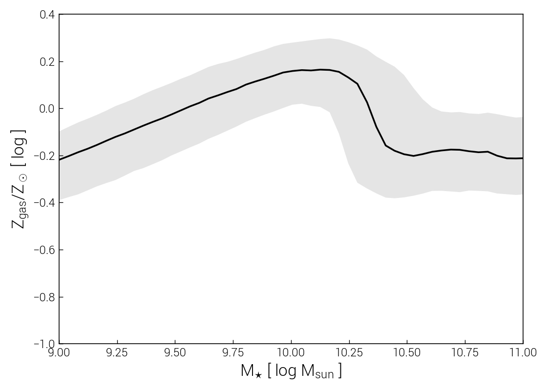
Let’s examine a classic observed galaxy scaling relation: the correlation between gas-phase metallicity, and stellar mass, the “mass-metallicity relation” (MZR):
sim = temet.sim(run='tng300-1', redshift=0.0)

temet.plot.subhalos.median(sim, 'Z_gas', 'mstar2')
This produces a PDF figure named median_TNG100-1_Z_gas-mstar_30pkpc_cen.pdf in the current working
directory. It shows the mass-metallicity relation of TNG100 galaxies at \(z=0\), and looks like this:
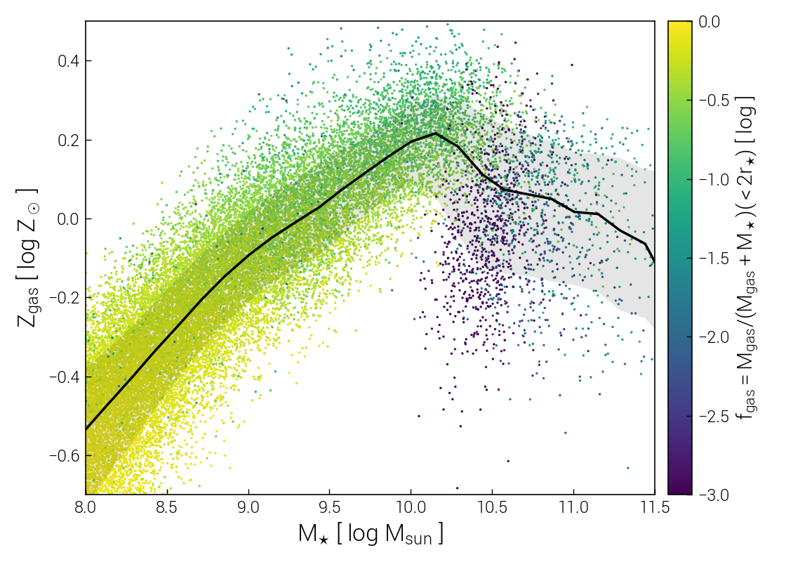
We can enrich the plot in a number of ways, both by tweaking minor aesthetic options, and by including additional information from the simulation. For example, we will shift the x-axis bounds, and also include individual subhalos as colored points, coloring based on gas fraction:
sim = temet.sim(run='tng100-1', redshift=0.0)

temet.plot.subhalos.median(sim, 'Z_gas', 'mstar2', xlim=[8.0, 11.5], ylim=[-0.7, 0.5], scatterColor='fgas2')
This produces the following figure, which highlights how lower mass galaxies have high gas fractions of nearly unity, i.e. \(M_{\rm gas} \gg M_\star\), and that gas fraction slowly decreasing with stellar mass until \(M_\star \sim 10^{10.5} M_\odot\). At this point, the overall gas metallicity turns over and starts to decrease, as indicated by the black median line. Gas fractions also drop rapidly, reaching \(f_{\rm gas} \sim 10^{-4}\) before starting to slowly rise again. This feature marks the onset of galaxy quenching due to supermassive black hole feedback.
Once you add a custom calculation for a new property of subhalos, i.e. compute a value which isn’t available by default, you can use the same plotting routines to understand how it varies across the galaxy population, and correlates with other galaxy properties.
Exploratory Plots for Snapshots
Similarly, plot.snapshot provides general plotting routines focused on snapshots,
i.e. particle-level data. These are also then suitable for non-cosmological simulations.
Functionality includes 1D histograms, 2D distributions, median relations, and radial profiles.
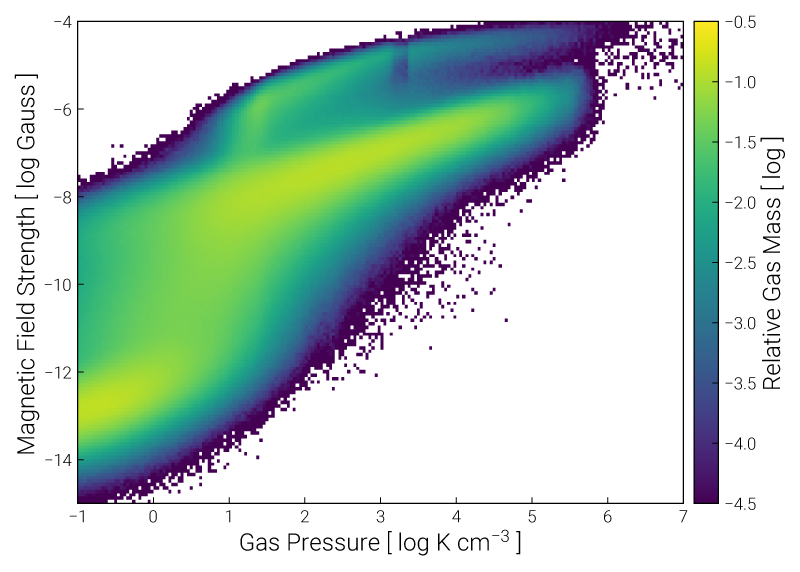
For example, we could plot the traditional 2D “phase diagram” of density versus temperature. However, we can also use any (known) quantity on either axis. Furthermore, while color can represent the distribution of mass, it can also be used to show the value of a third particle/cell property, in each pixel. Let’s look at the relationship between gas pressure and magnetic field strength at \(z=0\):
sim = temet.sim(run='tng100-3', redshift=0.0)

temet.plot.snapshot.phaseSpace2d(sim, 'gas', xQuant='pres', yQuant='bmag')
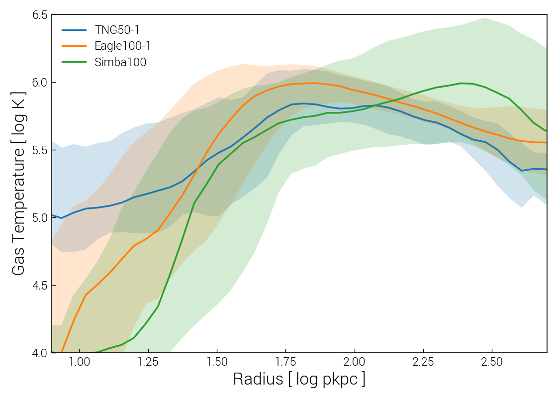
For cosmological simulations, we can also look at particle/cell properties for one or more (stacked) halos. For example, the radial profiles of gas temperature around Milky Way-mass halos, comparing TNG50, EAGLE, and SIMBA at \(z=0\):
sims = [temet.sim('tng50-1', redshift=0.0),
        temet.sim('eagle', redshift=0.0),
        temet.sim('simba', redshift=0.0)]

subIDs = []
for sim in sims:
    m200 = sim.subhalos('m200c_log')
    ids = np.where((m200 > 12.0) & (m200 < 12.1))[0]
    subIDs.append(ids)

temet.plot.snapshot.profilesStacked1d(sims, subhaloIDs=subIDs, ptType='gas', ptProperty='temp', xlim=[0.9,2.7], ylim=[4, 6.5])
As another example, the 2D phase space of (halocentric) radial velocity and (halocentric) distance, for all dark matter particles within the tenth most massive halo of TNG50-1 at \(z=2\):
sim = temet.sim(run='tng50-1', redshift=2.0)
haloIDs = [9]

opts = {'xlim':[-0.6,0.3], 'ylim':[-500,500], 'clim':[-4.7,-2.3], 'ctName':'inferno'}
temet.plot.snapshot.phaseSpace2d(sim, 'dm', xQuant='rad_rvir', yQuant='vrad', haloIDs=haloIDs, **opts)
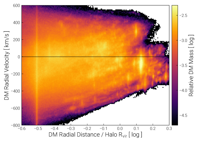
Here we see individual gravitationally bound substructures (subhalos) within the halo as bright vertical features.
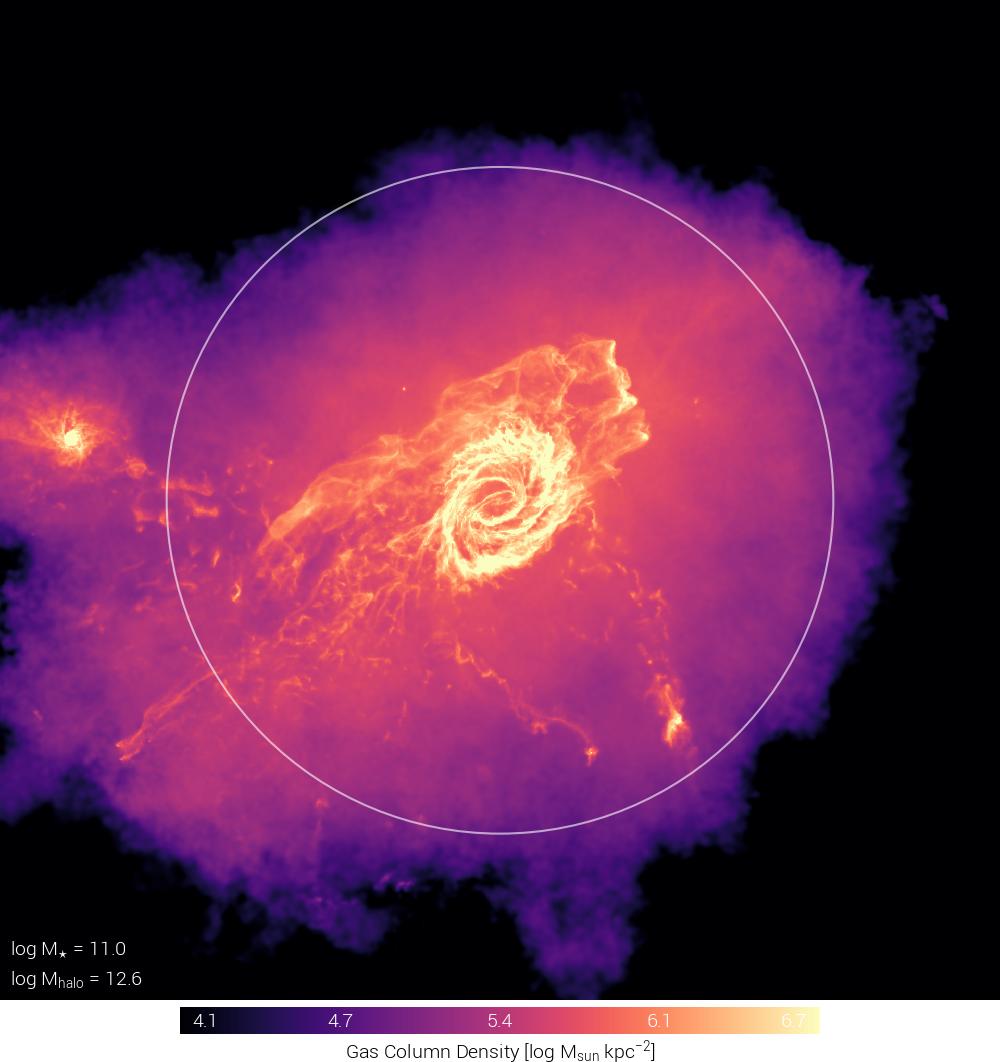
Visualizing a Halo and its Galaxy
We can request a visualization of any known snapshot quantity, with a large number of options.
For example, a projection of gas density on the scale of a dark matter halo:
sim = temet.sim(run='tng50-1', redshift=0.0)
subID = sim.halo(50)['GroupFirstSub']

# overall figure config
config = {'plotStyle': 'edged'}

# common variables shared between all panels
common = {'sP': sim, 'partType': 'gas', 'partField':'coldens_msunkpc2', 'labelHalo':'mhalo,mstar'}

# define panels
panels = [{'subhaloInd':subID}]

temet.vis.halo.renderSingleHalo(panels, config, common)
The images (or “panels”) in a figure are always specified by panels, a list of dictionaries. Each dictionary
specifies the options for that particular panel. Any option not specified will take the common value from common,
if present, or else a default value.
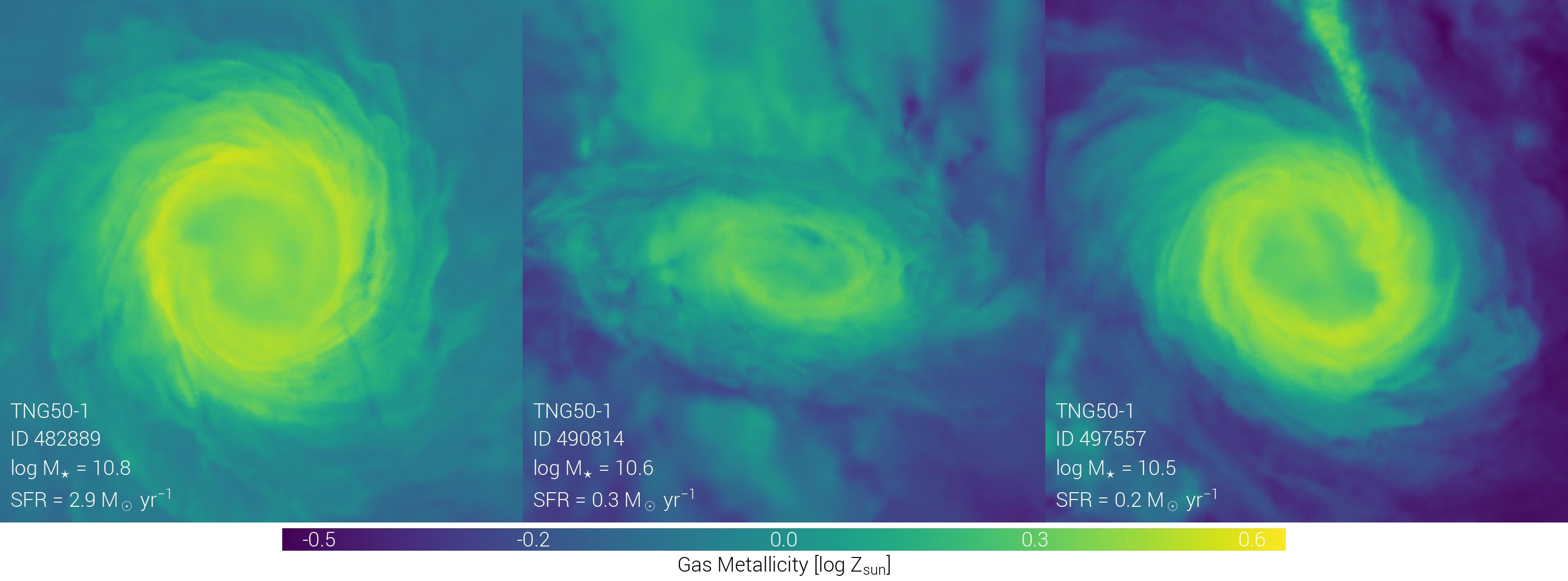
Or comparisons of gas-phase metallicity for several galaxies:
sim = temet.sim(run='tng50-1', redshift=0.0)

haloIDs = [120, 130, 140]

# overall figure config
config = {'plotStyle': 'edged'}

# common variables shared between all panels
common = {'sP':sim, 'size':0.2,
          'partType': 'gas', 'partField':'Z_solar', 'valMinMax':[-0.5, 0.6],
          'labelHalo':'mstar,sfr,id', 'labelSim':True}

# define panels
panels = []

for haloID in haloIDs:
    panels.append({'subhaloInd': sim.halo(haloID)['GroupFirstSub']})

temet.vis.halo.renderSingleHalo(panels, config, common)
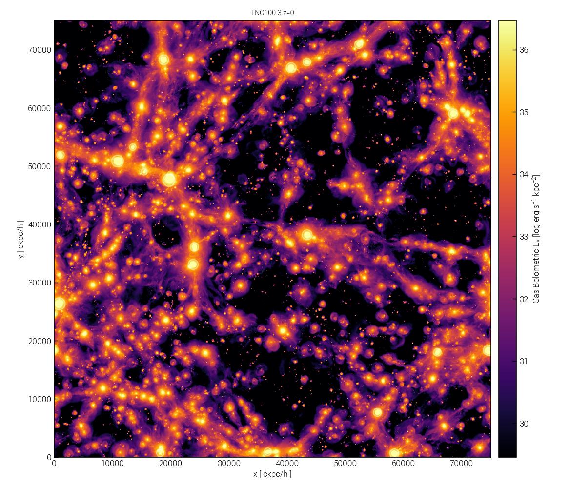
We can also visualize an entire box:
sim = temet.sim(run='tng100-3', redshift=0.0)

panels = [{'sP':sim, 'partType':'gas', 'partField':'xray_lum'}]

temet.vis.box.renderBox(panels)
The temet.vis.halo.renderSingleHalo() and temet.vis.box.renderBox() functions both accept dozens
of arguments that control the details of the visualization. These can vary for each and every panel. The simulation
sP can also vary by panel, allowing for comparisons between simulations and/or snapshots. In addition, there
are also global options that apply to all panels. See the Visualization documentation for details.
Note
The temet.vis.halo.renderSingleHalo() and temet.vis.box.renderBox() functions also have analogs
temet.vis.halo.renderSingleHaloFrames() and temet.vis.box.renderBoxFrames() that are
designed to automatically create a series of frames for movies.
Defining a Custom Field
So far we have been exclusively exploring and visualizing existing data directly available in the catalogs (e.g. galaxy stellar mass, galaxy size) or snapshots (e.g. gas density, magnetic field strength).
Often, additional quantities of interest can be directly derived from these existing fields. For instance, while gas temperature is often not stored in snapshots, it can be derived from internal energy.
We can define new “custom fields”. These are computed on-the-fly, when requested. To do so, a Python function containing the operational definition should be decorated as:
from temet.load.groupcat import catalog_field

@catalog_field
def my_ssfr(sim, field):
    """ Galaxy specific star formation rate, instantaneous (total subhalo SFR normalized by fiducial stellar mass)."""
    sfr = sim.subhalos("SubhaloSFR") # Msun/yr

    mstar = sim.subhalos("SubhaloMassInRadType")[:, sim.ptNum("stars")] # code mass
    mstar_msun = sim.units.codeMassToMsun(mstar)

    ssfr = sfr / mstar_msun

    return ssfr

my_ssfr.label = r"My sSFR"
my_ssfr.units = r"$\rm{yr^{-1}}$"
my_ssfr.limits = [-13.3, -8.0]
my_ssfr.log = True
Here we have defined a new field, my_ssfr, the galaxy specific star formation rate (sSFR), which is the total
instantaneous star formation rate (measured within the entire subhalo) divided by stellar mass (measured within
twice the stellar half mass radius). The four lines at the end assign metadata and plot units: a label, the units
of the return, suggested plot limits, and whether or not the quantity should be plotted on logarithmic axes.
We can then request a plot that includes this new field:
sim = temet.sim(run='tng300-1', redshift=0.1)

temet.plot.subhalos.histogram2d(sim, 'my_ssfr', 'mstar2', cQuant='fgas2', cRel=[-0.3,0.3,True])
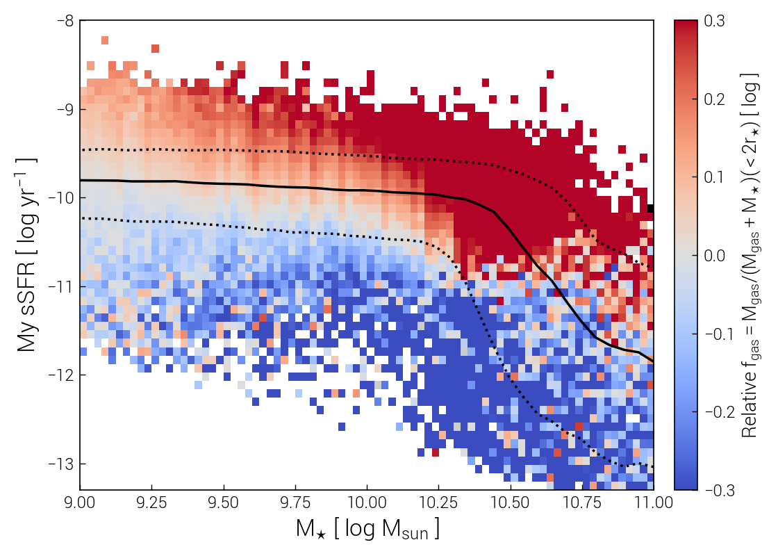
This is an example of a custom field defined for the group catalog, i.e. for subhalos. Similarly, custom fields can be defined for snapshot quantities, i.e. fields of particles/cells, with the temet.load.snapshot.snap_field decorator.
Computing a Custom Post-processing Catalog
Another common analysis task is to compute new properties for each object in a group catalog (halo/galaxy). Full details are provided in Catalogs.
Let us consider a simple example: to compute the total dark matter mass within 1 pkpc, for all subhalos. This value is not available in the default group catalogs, but can be easily computed from the snapshot:
from functools import partial
from temet.catalog.subhalo import subhaloRadialReduction

my_func = partial(subhaloRadialReduction,ptType='dm',ptProperty='Masses',op='sum',rad=1.0)
We then add this to the dictionary of available catalog definitions, giving it a sensible name:
from temet.load.auxcat_fields import def_fields

def_fields['Subhalo_Mass_1pkpc_DM'] = my_func
Note
The names of custom catalogs are left as a choice of the user, rather than being automatically generated, to make it easy to find (and possibly distribute to collaborators) the resulting files.
The first time we request this catalog, it will be computed and automatically saved to disk:
sim = temet.sim(run='tng100-2', redshift=0.0)

ac = sim.auxCat('Subhalo_Mass_1pkpc_DM')
Note
Such calculations range from fast to extremely expensive, in terms of compute time and memory usage. Many built-in
generating functions support an automatic chunk-based approach, that enables parallelization (on one node, or as
separate jobs spanning different nodes on a cluster) while reducing the memory requirement for each sub-calculation.
If the principal goal is to reduce memory usage, auxCat() can be replaced by auxCatSplit().
See Catalogs for details.
The result can be examined:
print(ac['Subhalo_Mass_1pkpc_DM'])

array([9.33235  , 9.307527 , 9.409516 , ..., 7.7760477, 7.7760477,
   7.7760477], dtype=float32)
We can then use this new catalog in any subsequent analysis or plotting, just like built-in fields. To do so, we need to define a custom group catalog field that handles loading and unit conversion:
from temet.load.groupcat import catalog_field

@catalog_field
def dm_mass_1kpc(sim, field):
    """ Dark matter mass within a spherical (3D) aperture of 1 pkpc."""
    acField = "Subhalo_Mass_1pkpc_DM"

    vals = sim.auxCat(acField)[acField]  # code mass

    return sim.units.codeMassToMsun(vals)

dm_mass_1kpc.label = r"$\rm{M_{DM}(<1 pkpc)}$"
dm_mass_1kpc.units = r"$\rm{M_\odot}$"
dm_mass_1kpc.limits = [7.4, 9.6]
dm_mass_1kpc.log = True
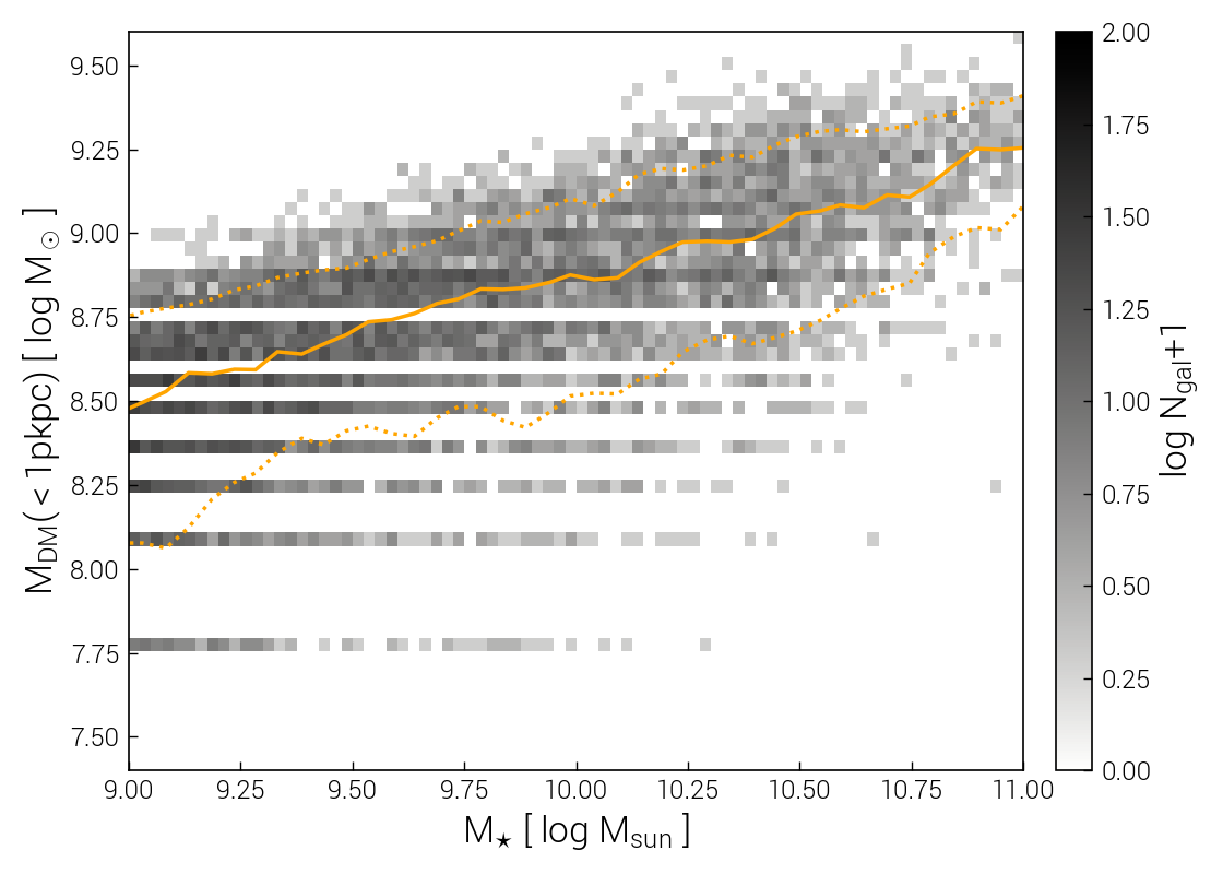
We can examine how the inner dark matter mass correlates with total stellar mass:
temet.plot.subhalos.histogram2d(sim, 'dm_mass_1kpc', 'mstar2')
Next Steps
You should have a feel for how to get started with temet now. The Cookbook of Examples contains further examples.
The remainder of the documentation describes in more detail:
loading data.
plotting.
visualization.
physical quantities and defining custom fields.
generating catalogs.
advanced topics.