Cookbook of Examples
Galaxy/Halo Catalog Queries
1. How many galaxies are there with stellar masses similar to the Milky Way?
sim = temet.sim("tng50-1", redshift=0.0)

# load
mstar_30pkpc = sim.subhalos("mstar_30pkpc_log")

# select
inds = np.where( (mstar_30pkpc > 10.5) & (mstar_30pkpc < 10.8) )[0]

print(f'In {sim} there are {len(inds)} such galaxies.')
In TNG50-1 (z=0.0, snapshot 99) there are 580 such galaxies.
2. How many central galaxies with \(10^{-11} < \rm{sSFR/yr} < 2 \times 10^{-11}\) exist?
sim = temet.sim("tng100-1", redshift=0.0)

# load
cen_flag = sim.subhalos("cen_flag")
ssfr = sim.subhalos("ssfr") # 1/yr, within twice the stellar half mass radius

# select
inds = np.where( cen_flag & (ssfr > 1e-11) & (ssfr < 2e-11) )[0]

print(f'In {sim} there are {len(inds)} such galaxies.')
In TNG100-1 (z=0.0, snapshot 99) there are 1282 such galaxies.
3. How many satellite galaxies with \(M_\star > 10^9 M_\odot\) exist in the TNG100 clusters?
sim = temet.sim("tng100-1", redshift=0.0)

# load
cen_flag = sim.subhalos("cen_flag") # equals zero for satellites
host_m200 = sim.subhalos("mhalo_200_parent_log") # log msun

# select
min_cluster_mass = 14.0 # log msun
inds = np.where( (cen_flag == 0) & (host_m200 > min_cluster_mass) )[0]

print(f'In {sim} there are {len(inds)} such satellite galaxies.')
In TNG100-1 (z=0.0, snapshot 99) there are 109806 such satellite galaxies.
Alternatively, and more directly:
sim = temet.sim("tng100-1", redshift=0.0)

# load
cen_flag = sim.subhalos("cen_flag") # equals zero for satellites

SubhaloGrNr = sim.subhalos("SubhaloGrNr") # the index of the parent group
GroupM200 = sim.halos("Group_M_Crit200") # code units
host_m200 = sim.units.codeMassToLogMsun( GroupM200[SubhaloGrNr] )

# select
min_cluster_mass = 14.0 # log msun
inds = np.where( (cen_flag == 0) & (host_m200 > min_cluster_mass) )[0]

print(f'In {sim} there are {len(inds)} such satellite galaxies.')
In TNG100-1 (z=0.0, snapshot 99) there are 109806 such satellite galaxies.
Particle/Cell Snapshot Queries
1. What is average star particle age in the entire simulation?
sim = temet.sim("tng100-1", redshift=0.0)

# load
ages = sim.stars("stellar_age")

print(f'In {sim} the mean stellar age is {np.nanmean(ages):.2f} Gyr.')
In TNG100-1 (z=0.0, snapshot 99) the mean stellar age is 8.29 Gyr.
2. What is the number gas cells in the box versus redshift?
These primarily decrease with time as gas is converted into stars:
ptNum = sim.ptNum("gas")

for z in [10, 6, 4, 2, 1, 0]:
  sim = temet.sim("tng100-1", redshift=z)

  print(f'At {z = :.1f} there are {sim.numPart[ptNum]} gas cells.')
Practice Exercise Solutions
The “Quickstart Guide for Heidelberg Groups (MPIA/ITA)” suggests a number of exercises to get familiar with the Illustris[TNG] data. Here we provide an example of solutions to each using this package:
import temet
import matplotlib.pyplot as plt
We will work with TNG100-3 at \(z=0\) for convenience:
sim = temet.sim('tng100-3', redshift=0.0)
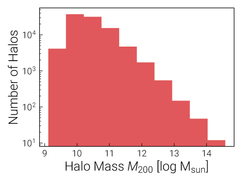
Exercise 0a
Choose one or two entries in the group catalog which sound interesting, and plot their distribution(s):
# load
m200 = sim.halos("Group_M_Crit200")
m200_logmsun = sim.units.codeMassToLogMsun(m200)

# plot
plt.hist(m200_logmsun)

plt.xlabel("Halo Mass $M_{\rm 200}$ [log M$_{\rm sun}$]")
plt.ylabel("Number of Halos")
plt.yscale("log")

plt.savefig("exercise_0a.pdf")
plt.close()
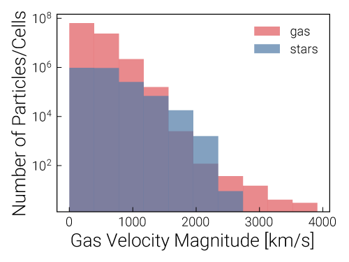
Exercise 0b
Choose one or two entries in the snapshot which sound interesting, and plot their distribution(s):
# load
gas_velmag = sim.snapshotSubsetP('gas', 'velmag') # km/s
stars_velmag = sim.snapshotSubsetP('stars', 'velmag')

# plot: automatic binning on first histogram, then keep bins constant for second
n, bins, _ = plt.hist(gas_velmag, alpha=0.7, label='gas')
plt.hist(stars_velmag, alpha=0.7, label='stars', bins=bins)

plt.xlabel("Gas Velocity Magnitude [km/s]")
plt.ylabel("Number of Particles/Cells")
plt.yscale("log")
plt.legend()

plt.savefig("exercise_0b.pdf")
plt.close()
Exercise 0c
Show the two-dimensional distribution, in space, of all halos in the simulation:
# load
pos = sim.halos("GroupPos")

x = pos[:,0]
y = pos[:,1]

# start a two-panel figure
fig = plt.figure(figsize=(12,5))

# in the first panel, use a scatterplot and rasterize the dots since there are so many
ax = fig.add_subplot(1,2,1)
ax.plot(x, y, marker='.', alpha=0.2, markersize=2, color='black', zorder=0)
ax.set_rasterization_zorder(1)

ax.set_xlabel("x [ckpc/h]")
ax.set_ylabel("y [ckpc/h]")
ax.set_xlim([0, sim.boxSize])
ax.set_ylim([0, sim.boxSize])
ax.set_aspect('equal')

# in the second panel, use a 2d histogram, which we show as an image
ax = fig.add_subplot(1,2,2)

hist_range = [[0, sim.boxSize], [0, sim.boxSize]]
h2d, _, _ = np.histogram2d(x, y, bins=50, range=hist_range)

h2d = h2d.T # careful with consistency with simulation coordinate system

extent = [0, sim.boxSize, 0, sim.boxSize]
im = ax.imshow(h2d, extent=extent, aspect='equal', origin='lower', interpolation='none')

ax.set_xlabel("x [ckpc/h]")
ax.set_ylabel("y [ckpc/h]")

plt.colorbar(im, label='Number of Halos')

fig.savefig("exercise_0c.pdf", dpi=300)
plt.close(fig)
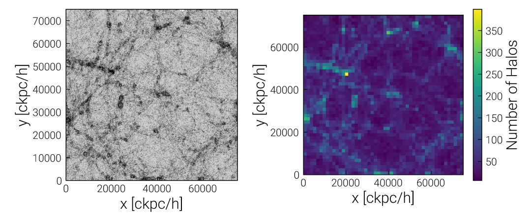
Note that we have chosen to plot the \((x,y)\) coordinates. By simply neglecting the \(z\) coordinate we are effectively projecting along the \(\hat{z}\) direction.
In the left panel we use a standard scatterplot, but this is rarely effective with large datasets, where crowding and overlapping can cause problems and/or be scientifically misleading. Instead the right panel uses a two-dimensional histogram to count the number of halos in each bin, and then visualizes this histogram as an image (with an automatic colormap and color scaling). A simple 2D histogram is often the most effective visualization choice.
Exercise 0d
Take the previous plot and use color, size, or symbol to show another property of each halo, such as mass:
# additional imports
from mpl_toolkits.axes_grid1 import make_axes_locatable
from scipy.stats import binned_statistic_2d

# load
pos = sim.halos("GroupPos")
mass = sim.halos("Group_M_Crit200")
mass_logmsun = sim.units.codeMassToLogMsun(mass)

x = pos[:,0]
y = pos[:,1]

# start a two-panel figure
fig = plt.figure(figsize=(12,5))

# in the first panel, use a scatterplot and rasterize the dots since there are so many
ax = fig.add_subplot(1,2,1)
s = ax.scatter(x, y, s=4, c=mass_logmsun, vmax=14.0, marker='.', zorder=0)
ax.set_rasterization_zorder(1)

ax.set_xlabel("x [ckpc/h]")
ax.set_ylabel("y [ckpc/h]")
ax.set_xlim([0, sim.boxSize])
ax.set_ylim([0, sim.boxSize])
ax.set_aspect('equal')

# colorbar
cax = make_axes_locatable(ax).append_axes('right', size='5%', pad=0.15)
plt.colorbar(s, cax=cax, label='Halo Mass [log $M_\odot$]')

# in the second panel, use binned_statistic_2d and filter out NaN values first
ax = fig.add_subplot(1,2,2)

hist_range = [[0, sim.boxSize], [0, sim.boxSize]]

w = np.where(np.isfinite(mass_logmsun))
c2d, _, _, _ = binned_statistic_2d(x[w], y[w], mass_logmsun[w], statistic='max', bins=100, range=hist_range)

c2d = c2d.T # careful with consistency with simulation coordinate system

extent = [0, sim.boxSize, 0, sim.boxSize]
im = ax.imshow(c2d, vmax=14.0, extent=extent, aspect='equal', origin='lower', interpolation='none')

ax.set_xlabel("x [ckpc/h]")
ax.set_ylabel("y [ckpc/h]")

cax = make_axes_locatable(ax).append_axes('right', size='5%', pad=0.15)
plt.colorbar(im, cax=cax, label='Halo Mass [log $M_\odot$]')

fig.savefig("exercise_0d.pdf", dpi=300)
plt.close(fig)
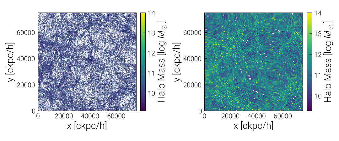
Here the right panel uses the binned_statistic_2d function to compute some statistic (such as mean, median, or max) on the data points which fall into each pixel (or bin). In contrast to the scatterplot on the left, where it is not clear what the color of many overlapping markers represents, we can precisely control the information content of the right image. Try experimenting with different statistics.
Exercise 1
Plot the relationship between galaxy sizes and galaxy stellar mass (and/or halo mass):
# load
mstar = sim.subhalos("mstar2_log") # within twice the stellar half mass radius [log msun]
size = sim.subhalos("rhalf_stars") # stellar half mass radii [pkpc]

# plot
fig = plt.figure()

ax = fig.add_subplot(1,1,1)
ax.plot(mstar, size, 'o', alpha=0.5, markersize=2, zorder=0)
ax.set_rasterization_zorder(1)

# draw median line
# todo: finish

# finish plot
ax.set_xlabel("Galaxy Stellar Mass [log $M_\odot$]")
ax.set_ylabel("Galaxy $R_{\\rm 1/2,\star}$ [pkpc]")
ax.set_yscale('log')

fig.savefig("exercise_1.pdf")
plt.close(fig)
Contributed Examples
Made an interesting analysis, plot, or visualization? Share it here!